Published on 28.11.2023

Chapter 1: Introduction to Random Walk

The initial encounter with stochastic calculus can be challenging, often appearing intricate and difficult to comprehend. This complexity can be attributed to certain prerequisites assumed by many introductory materials in the field. My goal here is to revisit this topic, starting from a foundational level accessible to those new to probability, with an emphasis on uncovering the inherent elegance of the subject.

In nature, complexity and simplicity are intricately linked, forming a unified whole. Each complex subject is composed of simpler elements, which in turn are built upon even more fundamental concepts. A “complex” phenomenon can be seen as a constellation of a more “simple” lower-level components. We can look at stochastic calculus through that lens: despite its apparent complexity, its foundation rests on straightforward, intuitive ideas from probability and statistics. To demonstrate this, we begin with the basics of binomial probabilities, which are fundamental to understanding the underlying structure of stochastic processes.

In the first posts, I want to walk through the very basics in binomial probabilities, introducing discrete-time random walk and illustrating how we can derive a Brownian motion process from it, which is fundamental to stochastic calculus and time series modeling in general.

Usually, probability theory is introduced with Bernoulli samples and the Binomial distribution: where the first one introduces the concept of a random variable, the second defines how we can use algebra to study the (discrete) random variable. This is the foundation, and the remaining theory evolves from it. Going with this theme, I’ll start in the same area but take a slightly different approach by focusing initially on the random walk, thereby examining the basics from a unique perspective.

Few things have an easier definition in math than it, since it literally means “the direction of each step is independently chosen by a flip of a coin.” You can easily simulate a random walk on your own by repeating the following procedure: Find an open space, preferably outdoors with space for 100 steps in both right and left directions (we’ll figure out why 100 later), and bring a coin with you.

As you arrive, take a coin and toss it. Then take a step to the right if it lands on heads, or to the left otherwise. Repeat this about 10,000 times (doctor’s recommendation for daily activity) to see where it can lead you. After some time, from wherever place you find yourself at, you can look at your journey and the destination as an unbiased, pure random movement.

If you plotted your journey on a graph with the x-axis representing time and the y-axis representing your relative location (zero indicates the origin), you would see something like this:

The first thing you’d probably notice is that you haven’t walked far away from your starting point. That’s not what would happen in your normal walk, where you generally stick to some direction while making a few turns here and there.
Mathematicians would tell you that your walk, which is a series of mutually independent events [1], has an expected value of zero: $\mathbb{E}[X]=0$ [2], and a constant variance $\text{VAR}[X] = \sigma^2$ [3] meaning you’d mostly stay within some fixed distance ($\sigma$) from the origin, not deviating away in one direction

These three properties are a mathematical way to describe hidden symmetry and structure in seemingly random, unrelated events.

Each independent step (coin toss) is completely unpredictable, unrelated to the rest, but if we look at the full walk, we can see a structure there.

Once I worked on a research project where I analyzed the prices of salvaged cars in dealerships across the US. I remember my first impression, the “wow” feeling when I looked at the distribution of millions of unrelated observations from places stretched out by thousands of miles, but still forming this beautiful symmetric shape.

Now, we can zoom back in to what makes a random walk random. For that, we want to look at what “fair coin” actually means.

In the context of probability, if someone mentions a “fair coin,” that means they’re talking about the Binomial distribution. It tells us how many times we can expect heads from a trial of nn tosses. And it does so by using a single elegant equation that is well-known in algebra:

$$(a+b)^n = \sum_{k=0}^{n}{n \choose k}a^{n-k}b^k = a^n + \ldots + n a b^{n-1} + \ldots + b^n$$

In this equation you can think of $a$ as a step right, and $b$ as a step left. Then, taking the $(a+b)$ to the power of number of steps $n$ produces the frequency of possible combinations of right/left steps one can make

One of the best way of visualisation that is by imagining a triangle where, each level represents the number of tosses, and the corresponding row represents the frequency expansion each possible right/left combinations.

Starting at the top, each row represents “information” about the distribution for each possible outcome at a given step:

At the initial step, there’s no outcome, hence 1:
$(a+b)^0 =1$
At the first step, we have either “head” (go left) or “tail” (go right), hence 1 and 1:
$(a+b)^1= 1 \times a + 1\times b$
At the second step, we have all information from the previous step plus a new step: one left-left, one right-right, and two left-right (note: because of the symmetry, we count left-right and right-left as equivalent since both result in the same point):
$(a+b)^2= 1 \times a^2 + 2 \times ab + 1 \times b^2$
The logic goes on.

With this in mind, we can combine both the “triangle” and “walk” trajectories into a combined view:

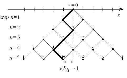
The numbers in the triangle now take on a new meaning: they quantify the various paths available for a walker to reach a certain location. For instance, in the illustrated graph, one can discern that there are ten separate paths leading to a chosen point, achievable within five steps.

Noticing the triangular shape, where the base grows linearly, it’s logical to deduce that the overall extent of the walk also increases in a linear fashion. Interestingly, this is mirrored in the variance, which accumulates steadily, at a rate of one unit per time period:
$$\text{VAR}(S_n)=n$$
Where:
$$
\begin{align}
S_n = \sum_{i=1}^nX_i \\
X = \begin{cases} +1 &\text{with probability} \frac{1}{2}, \\ -1 & \text{with probability} \frac{1}{2}, \end{cases}
\end{align}
$$

The logic becomes evident when considering the possibility of a direct path along the triangle’s edge – such as consistently moving left. In this scenario, after $n$ steps of this linear trajectory, you would be exactly $n$ steps from the starting point, a principle that applies to both directions. However, these straight paths are not common. Instead, our primary focus is on identifying the most likely outcomes. The triangle is useful in this regard too. By noting where the highest numbers accumulate, we can ascertain that they are generally close to the center and, importantly, they tend to cluster together!

To mathematically derive the measure of “average spread”, let’s recall that we have already established the variance of our random walk, ($\text{VAR}(S_n) = n$). The “average spread”, standard deviation, is defined as the square root of the variance. Hence, for our random walk, the standard deviation, denoted as ($\sigma$), is given by: [ $\sigma(S_n) = \sqrt{\text{VAR}(S_n)} = \sqrt{n}$ ] But why the square root? The square root is used because variance is calculated by squaring the deviations from the mean. This squaring process has a side effect of magnifying larger deviations. Therefore, to bring our units back to the original scale (as in our random walk), we take the square root of the variance.

Plugging the doctor-recommended walk $n=10,000$$$\sigma = \sqrt{n \text{VAR}(X)}=\sqrt{ 10,000}$$
We get $\sigma=100$, which align with your observations. It tells you how far from the mean (origin) you should expect to deviate.

An interesting feature here is the enduring nature of time symmetry, observable not only from the starting point but also at any point in the timeline. This means that, at point $x$ during time step $t$, the expectation of returning to $x$ persists, no matter the extent of the future projection from that point.

That means that if you cut off the historically observed trajectory of the walk, essentially forgetting it, you’ll end up with a new random walk, but centered at your current step. Repeating this at each step, you discover that each time you restart the walk with no memory of the past. This time series is known in the industry as a Markov chain.

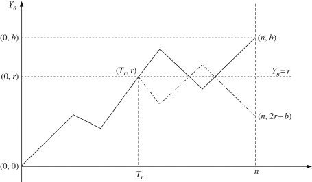
The illustration above shows that the random walk that starts at $(T_r,r)$ is statistically indistinguishable from the one that started at the origin $(0,0)$, i.e. we’d not notice any differences if we’d move the dotted $(T_r,r)$ walk back to the origin.

As we move to the next chapter, our focus will shift to a more detailed examination of symmetry. Reflecting on our learnings from this chapter, particularly the aspects of time symmetry and the behavior of the random walk, we’ll investigate how symmetry presents itself in various forms.

References:

- “Symmetric Random Walk - an Overview | ScienceDirect Topics.” n.d. Accessed November 27, 2023. https://www.sciencedirect.com/topics/mathematics/symmetric-random-walk.
- “Random Walk.” 2023. In Wikipedia. https://en.wikipedia.org/w/index.php?title=Random_walk&oldid=1186796458.