The Maker-Taker Coin Game: A Statistical Look at Prediction Market Pricing Part 1

Maker-Taker Coin Game

You’re at the boring party looking for ways to kill time. You’re with your friends Alice and Bob, and you invent a game that only requires a bag of coins and a little bit of math…

The setup is simple:

You have a bag of $n$ coins and all of them are weighted. Only you know the true probability $p$ of each coin landing heads, but Alice and Bob do not. Alice picks head, Bob picks tail. You’ll flip each coin once, for a total of n flips. On each flip Alice and Bob jointly contribute some amount to the bank total to $1. They need to agree on the contribution split, i.e. what portion pays Alice and what Bob.

Alice is more calm passionate. She think in terms of the distribution of outcomes, she proposes the price split point. In financial markets, she is known to be a maker - a person who makes markets for a given asset. Bob is reactive to the offered price, he will somewhat randomly accept or reject the bet. He may have strong beliefs about the probability of heads of that particular coin, he follows his intuition. Either one can skip the round. If a coin lands heads, Alice wins the $1 pot, otherwise Bob wins it. This is a clear zero-sum game - the winner takes all.

How should Alice set a price for the flip? If the coin were a fair coin with a probability of head is ~50%, then it is obvious to Bob not to accept a price greater than 50 cents for tails. If both of them knew the true probability $p$ of the coin upfront, then Bob should not accept a bet for tails at a price that makes the expected value of his bet negative, i.e. pay more than $K^{\ast} =(1-p)$. That is what we call a fair game.

But how would they play the weighted coin game where they don’t know the probability $p$ upfront? And more importantly, how can they agree on the split point $K$. Let’s study the game from both player’s perspective.

Expected Value of a Single Bet

Let’s call the probability of landing heads $p$.

Let’s call $K$ the price Alice will pay to contribute to the game. Bob will pay $(1-K)$ respectively.

Outcome	Probability	Alice Profit	Bob Profit
Heads	$p$	$1-K$	$-(1-K)$
Tails	$1-p$	$-K$	$K$

Alice’s expected value is: \(EV_{Alice} = p(1 - K) + (1-p)(-K) = p - K\) Bob’s expected value is: \(EV_{Bob} = (1-p) \cdot K + p \cdot (-(1-K)) = K - p\)

The edge $\alpha$ in this game is the absolute mispricing between the agreed price and the true probability: \(\alpha = | K - p |= |\text{price paid} - \text{actual probability}|\) If Alice’s estimate of the true probability of head $\hat{p}$ better than the agreed price $K$, then Alice owns the edge, otherwise, Bob does.

Alice knows several things about the bag of coins:

• There’re many of them.
• Her goal is not to be correct on each and every bet, but be profitable in total.
• Some coins are similar to each other: they have similar size, shape, color, or weight.

Alice decides to place a similar price K for a similar coins, under the core assumption that similar coins have similar underlying probability p.

Let’s say, she observed M different groups. Being statistician, she decides to collect some basic statistics for each group.

Variance of a Single Bet

Since she knows that the true probability $p$ can be anywhere in $[0,1]$ \(p \sim \text{Uniform(0,1)}\) She wants to understand how her risk changes across different kind of bets: (1) low-probability of head, (2) fair-ish coins, (3) high-probability head. For a head bet at price $K$ her profit $X$ takes values $(1-K)$ with probability $p$ and $-K$ with probability $(1-p)$. 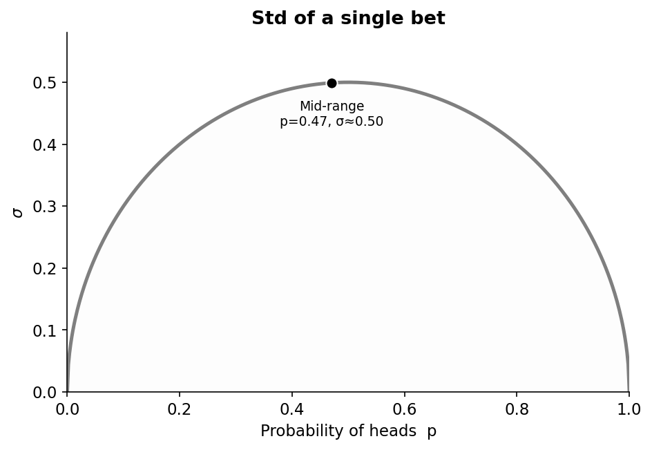Since \(X = Y - K\) \(Y \sim \text{Bernoulli}(p)\) the price $K$ drops out of the variance equation: \(\text{Var}(X) = \text{Var}(Y - K) = \text{Var}(Y) = p(1-p)\)

Region	$K$	$p$	$σ = \sqrt{p(1-p)}$
Longshots	0.10	0.07	0.26
Mid-range	0.50	0.47	0.50
Favorites	0.90	0.93	0.26

Variance peaks at $p ≈ 0.5$ and is lowest in the tails. Alice knows that she takes different risk for different types of coins - risk is almost twice as large near K~0.5 compare with the low/high ends of the range.

Alice decide to follow the strategy:

1. For the first $\widetilde{N}$ bets, she’ll doesn’t participate in the market, only observe outcomes for each coin, grouped in $M$ groups
2. Then, for each group, she computes empirical hit rate: \(\widehat{p_m} = \frac{\sum{X_m}}{N_m}\)
3. She selects only groups where $\widehat{p_m}$ is around $0.1$ or $0.9$, to minimize the payoff variance.

So what would be the realized payoff for Alice?

Realization Uncertainty

Both Alice and Bob want to get away with positive PnL. Bob decides he’ll bet aggressively and double down each time he loses so that the next bet will recover his PnL entirely. Alice adopts a different approach, she prefers steady but high probable cashflow, she thinks about this game more like a business rather than a gamble. For that to happen, she wants to have an answer for the following an important question:

Given the estimated probability $\widehat{p_m}$ and edge $\alpha= \widehat{p_m} - K$, how many bets $N_m$ does Alice need to place to have a high likelihood that her payoff will be positive?

With $N$ independent bets, the Central Limit Theorem gives us the approximation of the average payoff: \(\bar{X}_M \sim \mathcal{N}\left(\mu_M, \frac{\sigma^2}{N_{\text{M}}}\right)\) Where $\frac{σ}{\sqrt{N_M}}$ is the Standard Error $SE$ of the payoff mean. For Alice, the profitability condition for her game is that the lower bound of $CI > 0$: \(\mu - z_\alpha \cdot \frac{\sigma}{\sqrt{N_M}} > 0\) Solving for the minimum number of bets: \(\boxed{N_{\text{M}} > \left(\frac{z_\alpha \cdot \sigma}{\mu_M}\right)^2}\) Alice can use the formula above to determine how many bets she needs to place at a given edge $\alpha$ to lock the positive payoff.

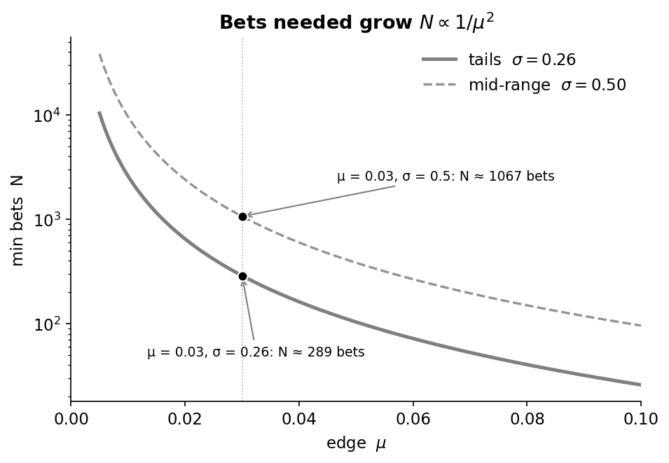
For example, suppose Alice estimates she has an edge of $\alpha=3\%$ for a high-likelihood low-risk coin (e.g. she places a bet price $K=0.87$ at the estimated $\hat{p}=90\%$). Then: \(\mu=\widehat{p}-K=0.03\) and if, using the lookup from the table above: \(\sigma \approx 0.26\) For Alice, to achieve profitability with 95% ($z_{\alpha} \approx 1.96$) confidence she needs to make at least:

\(N > \left(\frac{1.96 \times 0.26}{0.03}\right)^2 \approx 289 \text{ bets}\) To make the lower confidence bound of her PnL positive.

Below is the graph showing the relationship between min number of bets $N$ as a function of $\mu$:

She can even plot a surface showing how is the minimum number of bets needed varies in different price segments and edge buckets.

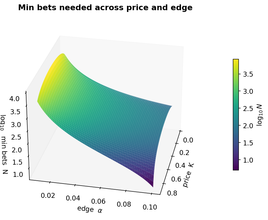
The $\frac{dN}{d\text{K}}$ price slope of this curve tells us how many more bets Alice need to make for a given change in the price. The $\frac{dN}{d\alpha}$ tells us how many fewer bets Alice needs to make for a step in the realized edge.

Calibration Curve

As Alice observes realized outcomes, she can track:

1. What was the expected hit rate for a given group of coins.
2. What was the actual hit rate.
3. How often Bob was willing to accept her bet price (since we’re not completely sure that Bob doesn’t keep record of the hit rate on his own)

Then, Alice can plot the price Bob accepted to pay against the historical hit rate.:

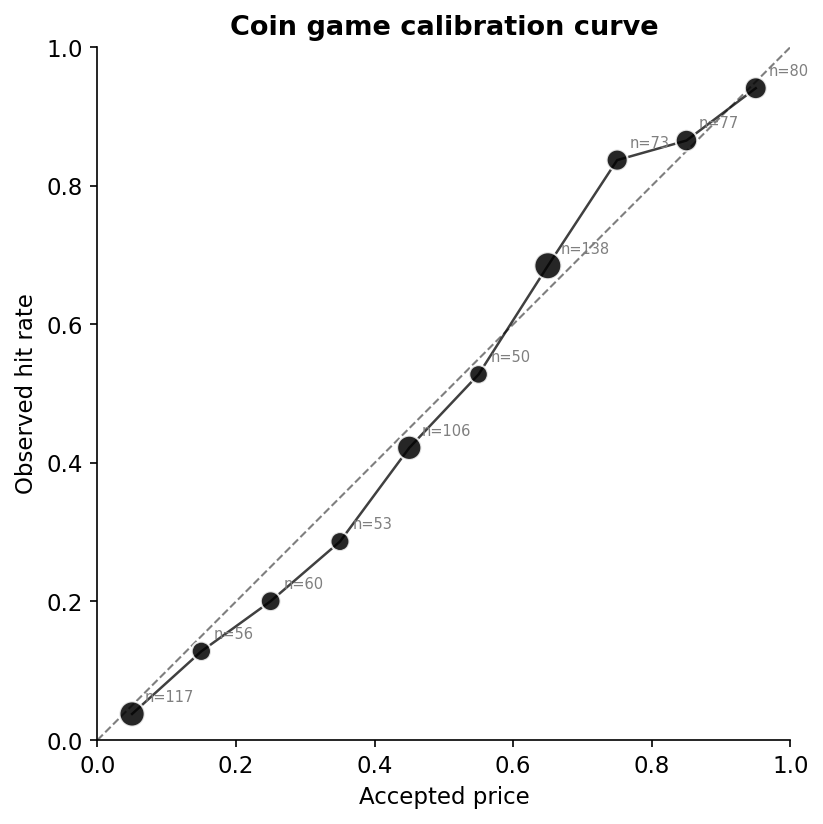
This curve is sometime referred as a calibration curve that measures how well the market-implied probability reflect the historical hit rate. In derivatives markets, option pricing models use a similar concept when comparing implied volatility against realized volatility.

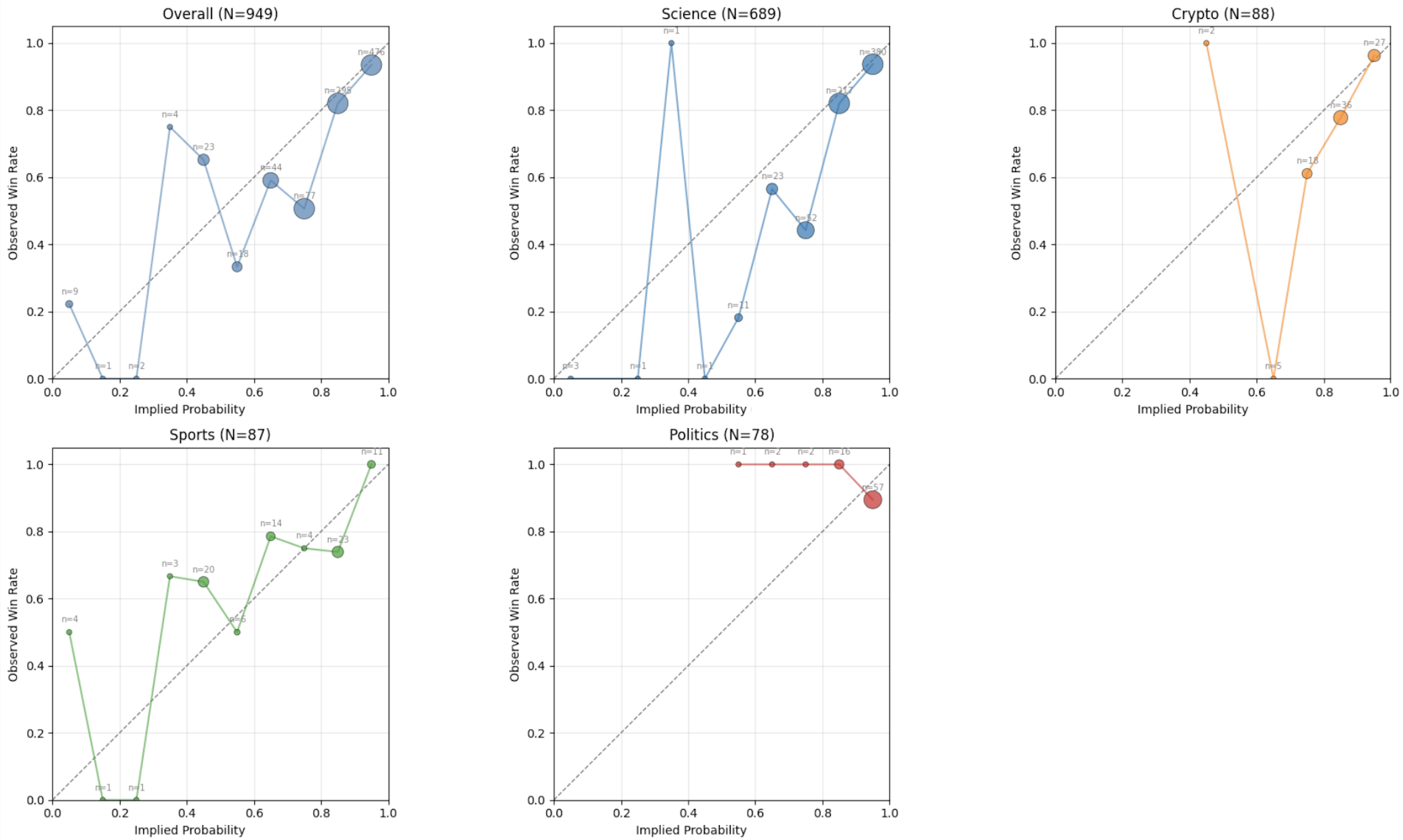
To get a little bit more practical here, the calibration curve gives a good leans on how prediction markets get priced. One can construct the curve by market category and study how well the market is calibrated. Perhaps, one can figure out a trading strategy based on that.

Here’s an example of the calibration curve of Polymarket prices split by category:

Maker vs Taker

We can study how simulated PnL of Alice and Bob evolves though time:

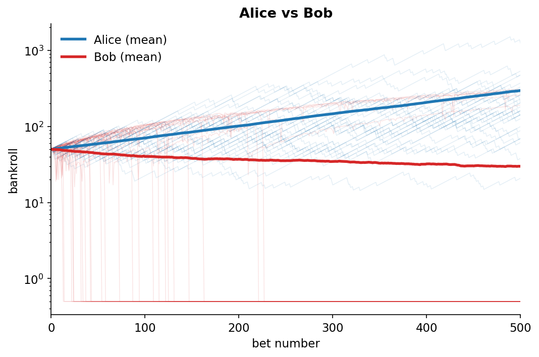
We can clearly see that starting at the same initial balance, Bob slowly but surely drains his bankroll whereas Alice slowly builds it up. In most of known markets uninformed, unsophisticated takers will drain their bankroll to makers. Their core difference is that they optimize different objectives:

Maker Alice optimize her cumulative PnL: \(\max_{\mathcal{B}} \; \mathbb{E}[\Pi_T]\) Where: \(\Pi_T=\sum_{t=1}^{T} X_t\) Alice only accepts bet groups $\mathcal{B}$ where the lower confidence bound is positive: \(\mu_m-z_\alpha\frac{\sigma_m}{\sqrt{N_m}}>0\) So her objective becomes: \(\max_{\mathcal{B}} \sum_{m \in \mathcal{B}} N_m \mu_m \quad \text{s.t.} \quad \mu_m-z_\alpha\frac{\sigma_m}{\sqrt{N_m}}>0\) Reactive taker Bob doesn’t apply any formal objective, so his behavior is random and governed by the volatility of his bets and his long-term survival is only possible, if the Alice systematically misprice her bets. In more realistic game, when players can set the size of the bet, as Bob accumulates losses, and start making impulsive, emotional judgments, he risks pushing himself to apply the martingale strategy to quickly recover losses. Unfortunately to him, this strategy is known to achieve gambler’s ruin under the finite bankroll with probability approaches 1.

For Alice, the more she in the market, the more the Law of Large Numbers (LoLN) materialize her edge. As we have seen earlier - more bets mean tighter confidence interval for her that eventually locks the positive pay-off. For Bob, the more he’s in the market, the greater the chance he’ll deplete his bankroll. The best possible strategy for Bob is to step away from the table when he got lucky and hit a positive streak.

Conclusion

The coin flip is just a hypothetical example, but estimation of the contract price on the prediction markets like Polymarket or Kalshi is not. This post gave a simplified example how one can use a basic statistics to study the price structure of the prediction markets. This approach can set a base for more sophisticated analysis needed for institutional strategies like basket trading or market making.

In the next post, we’ll go deeper and discuss how can one can incorporate uncertainty of the probability estimate $\hat{p}$, adjust the Effective Sample Size Under Correlation, and apply Kelly Criterion with Portfolio Weight Constraint.