Image credit geralt at pixabay
In this post we will talk about optimizing a simple portfolio of cryptocurrency. The approaches below have been successfully applied to stock options trading and, as we see, work quite well for crypto. Also, crypto is great to learn and try modern trading strategies as you can get required historical currency data for free (we will show how below). In this post we do a simple portfolio composition and apply CVXPY optimization to introduce library and methods and we will go into more complex Stochastic Discount Factor based strategies in the next post.
You are welcome to open our notebook on colab and see full working code, here we hide some technical parts.
Data Acquisition
The data for this exercise was obtained from the Binance API using the Python API client python-binance. While obtaining similar data for stock market would have been quite a task on its own (unless you work for a trading firm), in crypto worlds it is done easily.
An example of the data acquisition code:
Note: Install the module if needed using pip (pip install python-binance)
from binance.client import Client
binance_api_key = 'YOUR-API-KEY'
binance_api_secret = 'YOUR-API-SECRET'
binance_client = Client(api_key=binance_api_key
                ,api_secret=binance_api_secret)
klines = binance_client.get_historical_klines(symbol
                 ,kline_size, date_from, date_to)
data = pd.DataFrame(klines, columns = [COLUMNS])
Following daily pairs was downloaded and formatted to pd DataFrame:
- BTCUSDT
- ETHUSDT
- BNBUSDT
- LTCUSDT
For each timepoint, Binance provides conventional OHLC (Open, High, Low, Close) and Volume data. In this exercise, we used only the Close column. One might consider the combination of all five values and come up with a different (and potentially more reliable) metric, for example: the weighted average price. We will limit to the basic one for the sake of simplicity
The data is loaded and transformed:
fuldf = (pd.read_csv('https://raw.githubusercontent.com/h17/fastreport/master/data/cryptosdf/data.csv',parse_dates=['timestamp'])
        .set_index('timestamp')
        )
y_label = fuldf.columns[0]
factors = (fuldf
           .columns
            .tolist()
          )

total_size = fuldf.shape[0]

train_set = .8

train_id = int( total_size * train_set)
df_train = fuldf.iloc[:train_id]
df_test = fuldf.iloc[train_id:]
split_index = fuldf.iloc[train_id].name
The joint time-series of four crypto assets looks the following:
df_train.head()
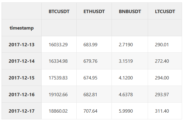
Each trading pair has a different amount of data available: The oldest tradable crypto instruments on Binance are BTCUSDT and ETHUSDT — data points are available from 2017–08–17. For BNBUSDT and LTCUSDT first trading days are 2017–11–06 and 2017–12–13, respectively.
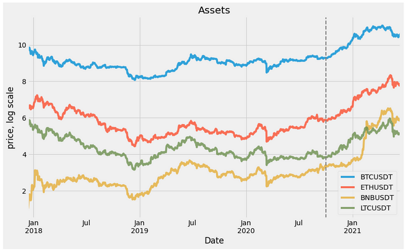
We joined these time series together on the earliest common trading date: 2017–12–13 up to 2021–06–14. The full joint dataset size is equal to 1280 samples. In order to properly train the model, We split the dataset into training and testing sets at 2020–10–02.
Training interval: 2017–12–13 to 2020–10–02 (1024 data points).
Below is the joint plot of the full dataset in the logarithmic scale. The dotted line represents the train-test split at 2020–10–02
plot_data =np.log(fuldf)
fig , ax = plt.subplots(figsize=(12,7))
plot_data.plot(ax=ax,alpha=0.8)
ax.legend(loc=0)
ax.set(title='Assets',xlabel='Date',ylabel='price, log scale');

ax.axvline(split_index,color='grey', linestyle='--', lw=2);
#Transform raw data to log-return format:
lret_data = np.log1p(df_train.pct_change()).dropna(axis=0,how='any')
Data Transformation
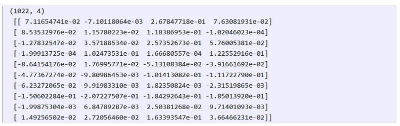
In order to be properly trained, input time series has to be transfored into the log-return format:
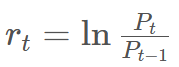
Where P_t is a price of the asset at time t. The model needs vector I to perform the optimization:
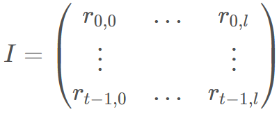
Where l is the number of features in the model.
I = (lret_data[factors].iloc[1:].values)

print(I.shape,'\n',I[:10,:])
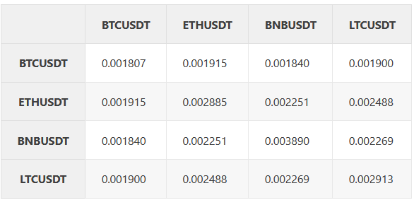
F = pd.DataFrame(I)
F.columns = factors#+ [y_label]
F.cov()
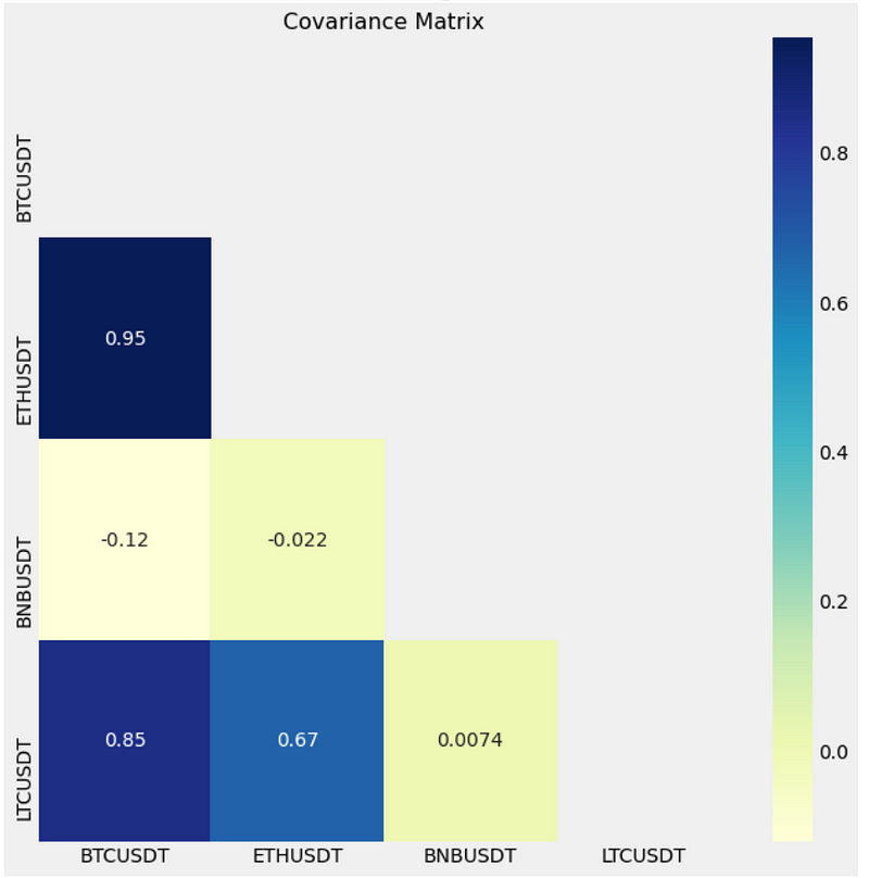
f = plt.figure(figsize=(10, 10))
cov_data = F.cov()
mask = np.triu(np.ones_like(cov_data))
dataplot = sb.heatmap(cov_data.corr(), cmap="YlGnBu", annot=True, mask=mask)
plt.title('Covariance Matrix', fontsize=16);
Model
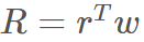
Our goal is to explain the differences in the cross-section of returns R for individual stocks.
Let I denote the return of crypto assets at time t. We try to obtain weights w that minimize risk given fixed return. The portfolio return R can be expressed as follows:
For this model portfolio, we target a 100% return, which is quite expected in the crypto world. We will only model investments held for one period.
The problem can be expressed as:
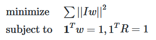
Since the above problem is convex, we can estimate the w for the model portfolio using the cvxpy framework.
Note: in reality, you want to get maximum return given fixed risk, but due to the way CVXPY and semi-linear programming is setup, this formulation does not follow Disciplined Convex Programming rules (see https://dcp.stanford.edu/), so we use the former formulation as it is equivalent. Also, you might need fix return and low risk models depending on type of business your are in and your risk appetite.
#define weights
w = cp.Variable(shape=(I.shape[1]
,1),nonneg=True)
#Define expression
R = I @ w
#Construct the problem
prob = cp.Problem(cp.Minimize( cp.norm(R) )
, [ cp.sum(R) == 1
,cp.sum(w) == 1
]
)
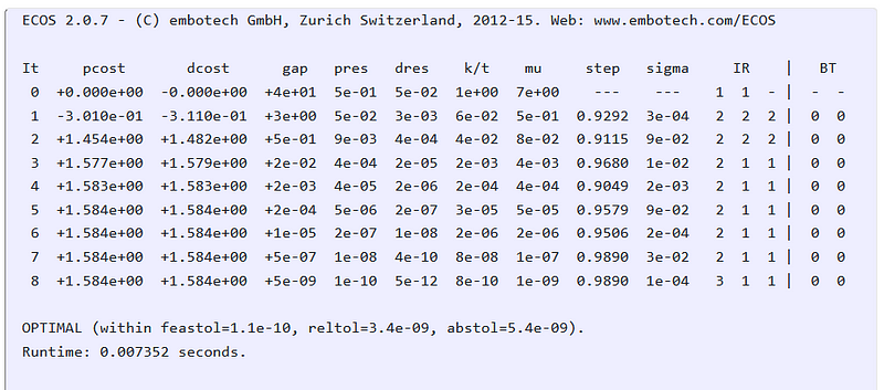
prob.solve(verbose=True)
print('weights for the model:\n',dict(zip(factors,w.value)))
CVXPY output for the optimization run:
Results
Let’s define utility functions to analyze our model portfolio:
def sharpe(x):
  return (x.mean() / x.std() * np.sqrt(365))

def calc_metrics(data):
  p_return = ((data[factors].pct_change().fillna(0))
              .apply(lambda x: (x @ w.value)[0] ,axis =1)
              .rename('Model Portfolio')
              )
  returns = data.pct_change().fillna(0)
  returns['Model Portfolio'] = p_return
  sharpes = returns.apply(np.log1p).apply(sharpe)
  pnls = (returns.apply(np.log1p).sum().apply(np.expm1)).apply(lambda x:f'{100*x:4.2f}%')
  result = pd.concat([sharpes,pnls],axis=1)
  result.columns='sharpes pnls'.split()
  return result

def plot_return(data,title):
  datac = data.copy()
  fig , ax = plt.subplots(figsize=(13,5))

  y_return = (datac[factors].pct_change().fillna(0)+1)

  p_return = ((datac[factors].pct_change().fillna(0) + 1)
              .apply(lambda x: (x @ w.value)[0] ,axis =1)
              .rename('Model Portfolio')
              )

  p_return_c = p_return.cumprod()
  y_return_c = y_return.cumprod()
  portfolio_benchmark = pd.concat([y_return_c,p_return_c],axis=1)

  #change to the log scale
  portfolio_benchmark = np.log1p(portfolio_benchmark)
  portfolio_benchmark[factors].plot(ax=ax,alpha=.5)
  portfolio_benchmark['Model Portfolio'].plot(ax=ax,alpha=.7,color='black')
  ax.legend(loc=0)
  ax.set(title=title,ylabel='growth factor',xlabel='date')

  return portfolio_benchmark
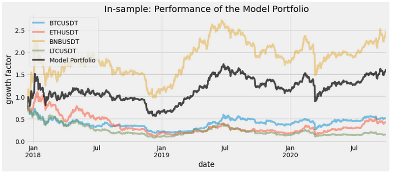
Below is the result of computing the Model Portfolio on the training dataset and plotting it against the index portfolio (BTCUSDT):
calc_metrics(df_train)
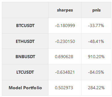
portfolio_benchmark = plot_return(df_train,'In-sample: Performance of the Model Portfolio')
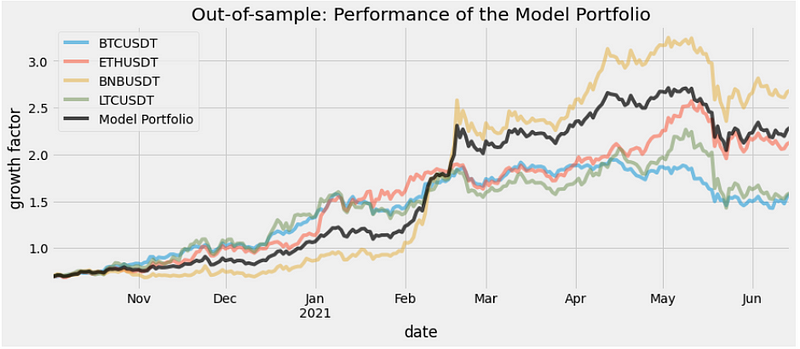
Resulted plot and metrics for the hold-out dataset:
calc_metrics(df_test)
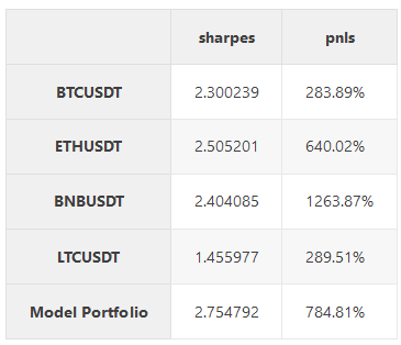
portfolio_benchmark_ho = plot_return(df_test,'Out-of-sample: Performance of the Model Portfolio')
Conclusion
In this exercise, we fixed the return of our portfolio and minimized the risk — we get better sharp than any of the coins and performance between best and second-best performing coin.
Disclaimer: authors of this paper do not use these methods for any investments and do not recommend to use this paper for investment. It is just for demonstration purposes of the CVXPY. The material presented here is done without a backtest, daily simulation or cutting-edge libraries. We would recommend to use MOSEK library and more rigorous approach.
Originally published at https://yourdatablog.com